At Grøft Design, we continuously seek interesting real-world problems within the industry. Our client, Norconsult, faced a interesting challenge they couldn’t solve with traditional methods:

Sizing power cables for a heavy-duty EV charging depot. The system operates through a substation using 32 power cables. Based on the historical data, during peak-hours with a full load, the charger delivers approximately 3.5 MW. This load may generate significant heat.

1. Steady state analysis: a conservative method commonly used in practice that assumes continuous operation at maximum load.
2. Cyclicload analysis : incorporating load factors to account for varying charging patterns.
3. High-resolutiontime-variable analysis : account for actual load-flow by simulation load, minute-by-minute.

Furthermore, by validating the Grøft Design model against measured temperature of cables on-site, we demonstrated how the cyclic load analysis provides an accurate solution,enabling cost-effective and reliable design of the EV charging infrastructure.

Step 1: Modelling the Shallow Duct-Bank

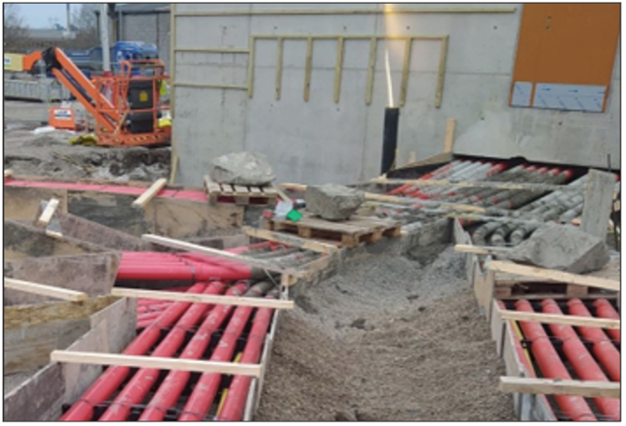
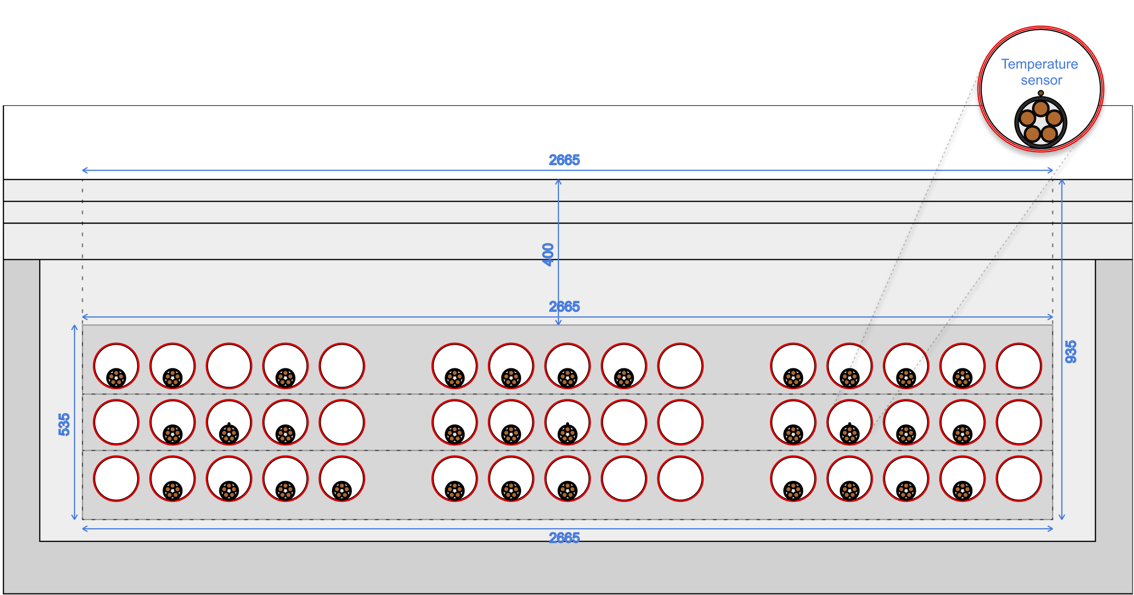
The first step involves modeling the installation – a shallow duct bank. In the software, multiple layers of different varying thermal parameters are modeled, reflecting the real installation conditions – surrounding soil, trench backfill, sub-grade, base and surface layer of a road over the concrete duct-bank. As part of our research projects we have studied soil conditions and created guidelines for selecting appropriate soil parameters.

Step 2: Selecting or Designing Cables

In Grøft Design you may design your own cable (https://docs.groftdesign.net/features/cable-designer/) according to the manufacturer's datasheet specification or select a typical EV charging power cable from the Grøft Design cable library for preliminary assessment of the installation.

Step 3: Install Virtual Sensors

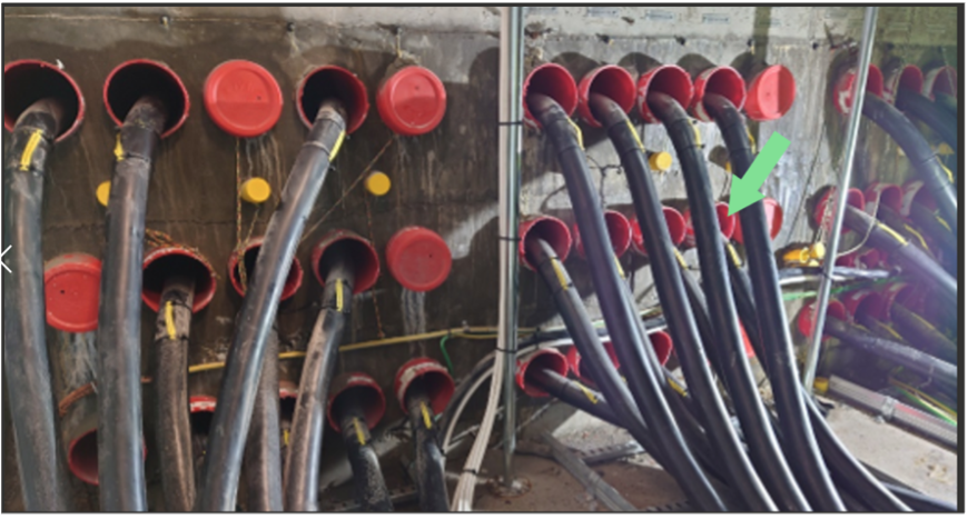
For the installation three cables were equipped with sensors mounted on the power cable jacket to measure temperature. In Grøft Design, virtual sensors can be placed anywhere in the trench to measure temperature and magnetic field in the model.  Later on, these virtual measurements can be used to validate and calibrate the model against the physical measurements.

‍

Step 4: Analyses

Case Study 1: Steady state analysis

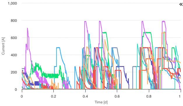
To analyze the system under continuous load, supply cables were assigned to corresponding chargers. Cables are grouped in sub-distribution units – each unit supplies two to three chargers; therefore, the current load on each unit is individual. Based on the historical data, the power being delivered during peak utilization of the chargers is approximately 3.5 MVA.

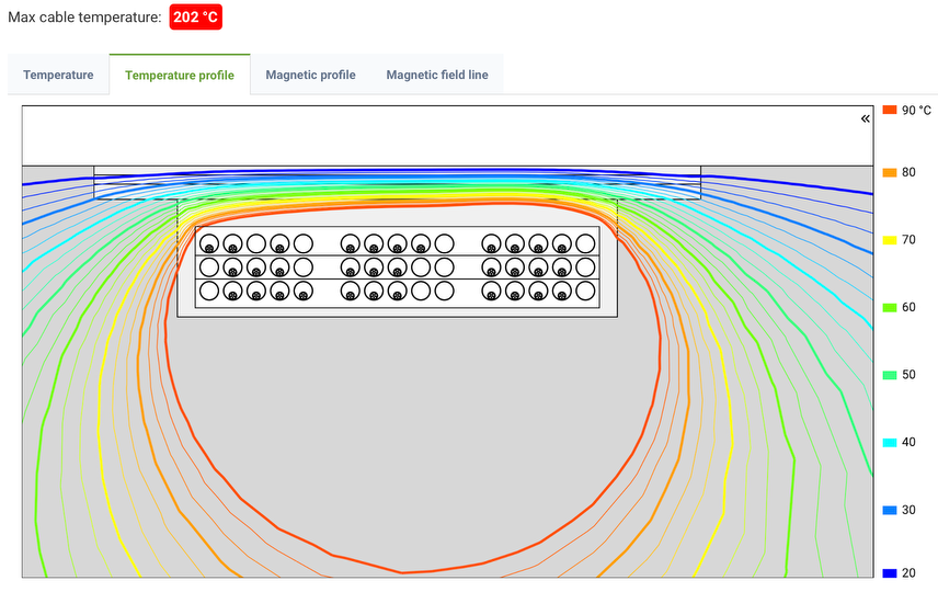
A steady-state analysis with this load results in maximum cable temperature of 202 °C, which dramatically exceeds the maximum allowable temperature for the cable. Furthermore, high temperature gradients are developed within the duct-bank section invalidating the physical assumptions underlying this model. Three primary mechanisms drive this elevated temperature:

• First, steady-state analysis produces conservative predictions by assuming indefinite simultaneous charging at all stations - an operationally unrealistic scenario.
• Second, thermal instability occurs when the conductor is near its thermal capacity, which amplifies temperature rise exponentially.
• Third, the constant ground surface temperature boundary condition poses physically inconsistent behavior in the duct-bank section, which acts as artificial cooling. Therefore, the boundary conditions at ground level should be changed to the reference air temperature instead. This is particularly relevant for shallow installations, as noted in IEC standards and Cigre TB 640. On hot summer days, asphalt pavement can reach temperatures of 50 - 60 °C, even in Norway!

Case Study 2: Dynamic load

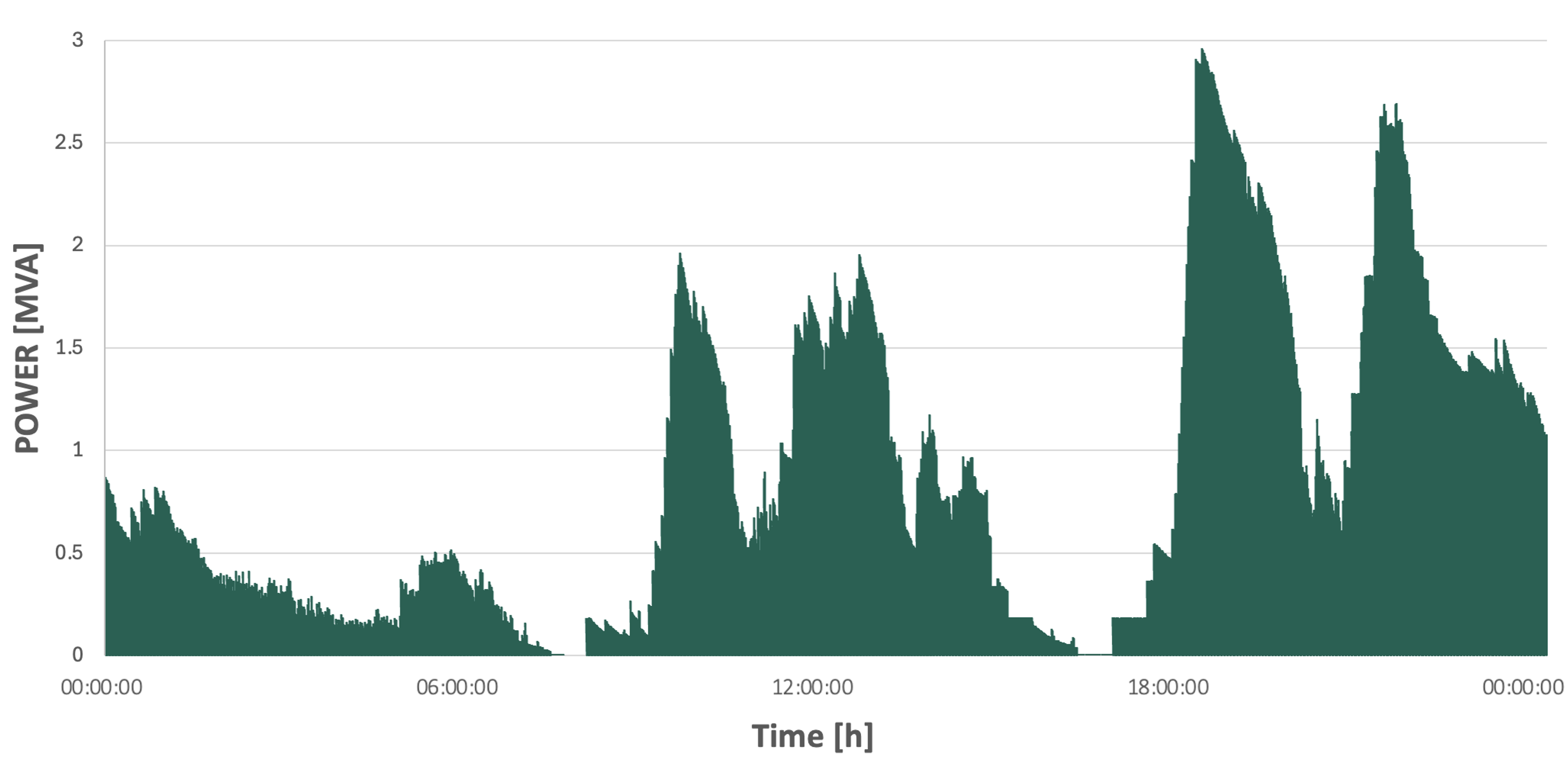
We analyzed charging data for the  EV charging depot, visualized in the graph below. These curves represent a typical charging day. It is noticeable when chargers are active simultaneously. The most active periodes are between 09:00 and 12:00 and between 18:00 and 21:00. During this window, the load reaches 2.8 MW for a short 3 to 4-hour period.

The measured temperatures on the three sensors that day were merely up to 31 °C. This is significantly lower than the indicative results of the steady-state Case Study 1.

Consequently, the advantage of applying Grøft Design for establishing the true current capacity of this facility will be highlighted here:

1. The record of the time-varying load current data is uploaded individually to the corresponding distribution units (time-series csv. or .txt file)
2. To increase the reliability of the current-rating analyses carried out in the software, we compared the measured on-site temperature data with the simulation model results, applying the same time-varying load current. This comparison  is useful while adjusting model parameters, such as thermal resistivities of soil, creating digital twin of the facility. This is a high-precision approach.
3. With a concrete duct bank and multiple cables having different load curves, running the analysis for a complete single day can take  considerable amount of time if we apply the uploaded one-minute resolution curves. Therefore, the software may modify the resolution of these loading curves to optimize the analysis time. For that case, 20 min resolution was chosen. See figures below.
4. It is crucial to examine the thermal conditions within the duct-bank at the start of the analysis. The initial steady-state analysis is run to achieve the same temperature on the virtual sensors as was measured in the field at the start of the time series. The alternative approach is to extend the analysis time to several days as the initial step, which increases accuracy while comparing the measured data, this though, may be computationally less effective. Furtheremore, fluctuations of the reference air temperature above ground level may be incorporating  in the analysis.

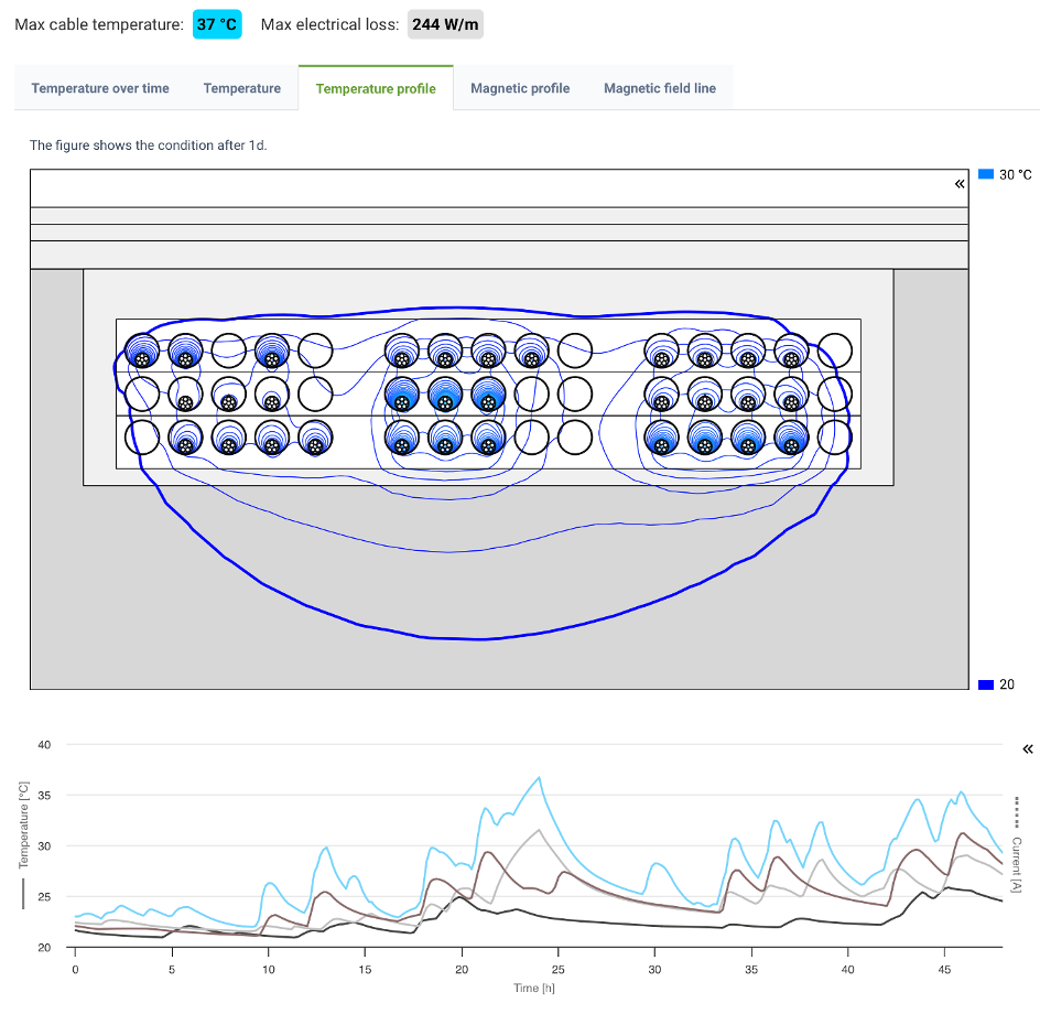
A comparison of measured vs. simulated temperatures at the probes is presented in the figures below. The sensor temperatures tracked on-site are represented with a dotted line, while the solid line represents the temperature simulated in Grøft Design. The difference for the initial temperature within the duct bank is highlighted by comparing the two figures, representing steady-state and dynamic approach, accordingly.

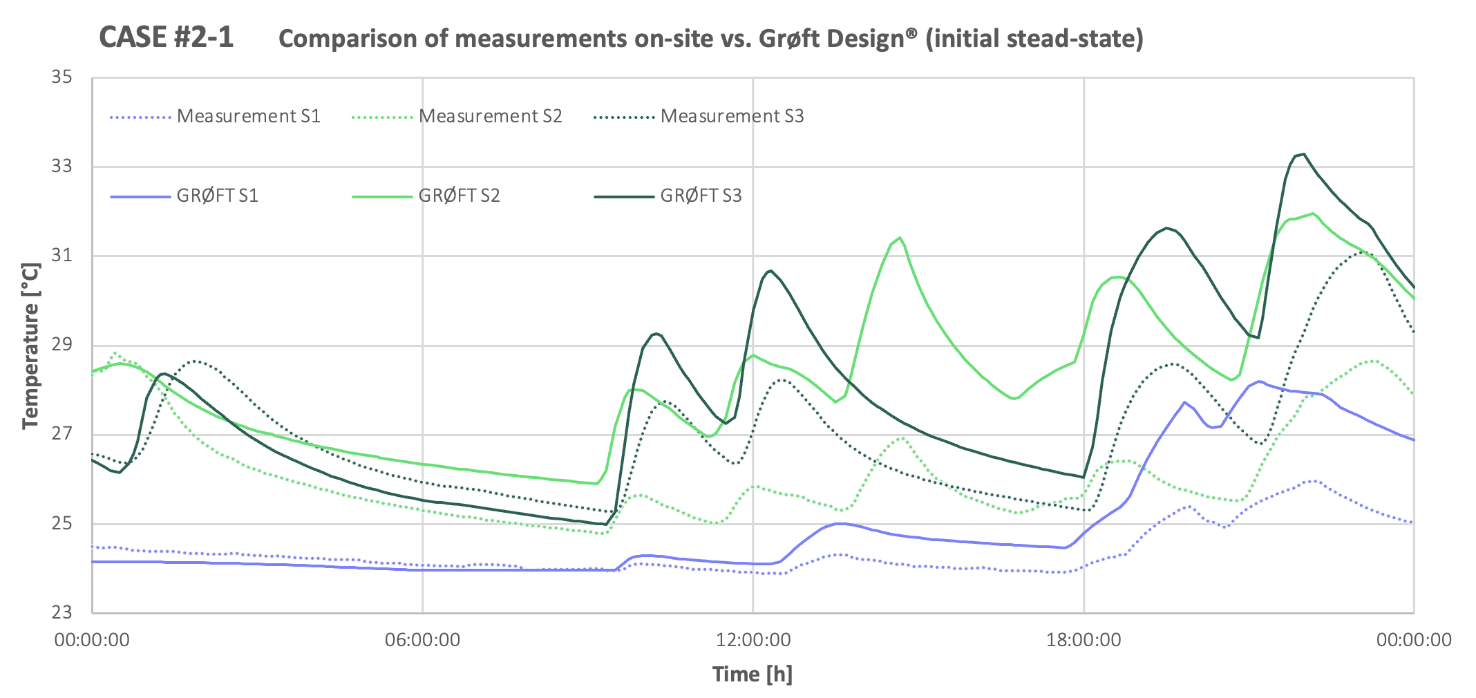
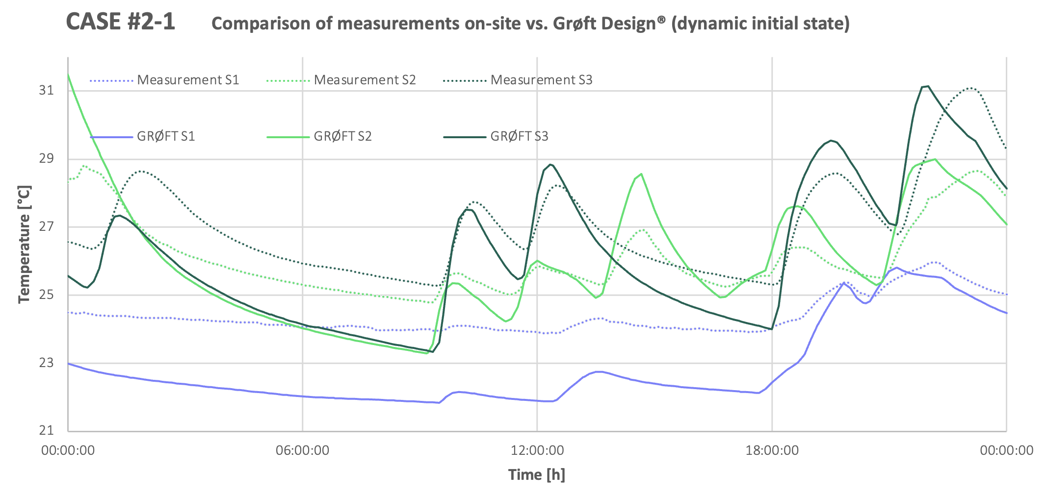
Application of both methods for the initial state is valid, and the accuracy of the temperature plots comparison with reference to the measurements performed on-site is very satisfactory. The maximum conductor temperature during this one-day cycle is 37 °C.

There are still several uncertainties in this model beyond facility specification, however, the result alignment is validated. In such, the simulated results incorporate are slightly conservative with reference to the measurements, satisfying the safety margins imposed on engineering assignments and risk-assessment. Such a validated model is further used for establishing the true current carrying capacity.

Case Study 3: Load Factor

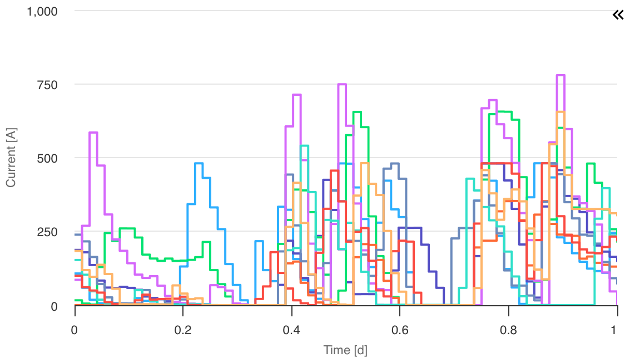
While the dynamic load application methodology provides the highest precision for establishing current ratings, it is computationally intensive. Engineers often prefer a more time-efficient approach: the load-factor methodology, implemented in Grøft Design software based on IEC standards. This approach analyzes the uploaded load curves to calculate the applicable load factor for the installation, which serves as input to the analysis.

Applying the worst-case load factor derived from the load curves, simultaneously dimensioning all cables to this maximum condition, represents the most reliable approach. This method satisfies the required safety margins for the facility while significantly reducing computation time. Results are now generated in minutes rather than hours.

Validation against on-site measurements confirms satisfactory correlation: the maximum conductor temperature is 46 °C. This result demonstrates substantial improvement over traditional steady-state analysis, and proves highly effective for the optimization process.

Case study 4: Maximum Cable Temperature at Full Load

Now that we have a model that aligns well with the reference conditions and actual load patterns, we can use the same model to calculate the maximum load for the facility. Based on the historical data, we found that the average load factor for the facility is approximately 0.3 and the maximum utility current is 210 A. By using load factor analysis, the simulation results with a maximum cable temperature around 70 °C -  well below 90°C, the maximum permissible temperature for this cable.

Summary

As seen in this case study, steady-state calculations often yield excessively conservative load limits. With Grøft Design's time-varying load analysis, we can choose the level of detail for the analysis that we want by combining temperature measurements with virtual sensors, air temperatures timeseries, different thermal resistivities in surrounding soils, soil drying effects, high-resolution time-varying load curves, or load factors for faster analysis. Grøft Design uses Finite Element Analysis, bypassing many of the limitations of traditional analytical models. With the possibilities in Grøft Design the limitation of the analysis is no longer the level of detail of the analysis, but the amount of information the engineer has regarding the installation, like actual load patterns and thermal conditions around the cables. Time to compute an analysis is also an important factor. Finding good ways to optimize is important, like changing time resolution of load curves or using load factors.

Grøft Design includes several unique features for time-variable load analysis.

• These include load curve pre-processing, where adaptive resolution algorithms efficiently manage high-frequency data while maintaining accuracy.
• Multiple options to select the initial condition of the analysis. In this case, we tried both steady state, and dynamic load from the hours before.
• It also features multi-cable analysis for simultaneous analysis of complex, multi-cable systems with individual load profiles.
• Finally, it offers a rich and user-friendly interface for drilling into the analysis results.

‍

Disclaimer: Each project requires a separate, individualized approach with a level of detail determined by the design engineers.